


[This post describes the mathematical analysis of the dynamics and unit economics of the standalone food delivery companies in India. For example, in order to arrive at monthly “burn rate” calculations (i.e., how much money the standalone food delivery companies are losing), we have used India-specific numbers for delivery charges and labor costs, among others. However, the mathematical models on order arrival rates, wait time and how they affect service levels, apply globally].
“Eating out” is out, “ordering in” is in. In this new convenience economy, the restaurant industry is learning to cope with this change with a host of startups providing new ways of delivering food to customers on demand. Investment has predictably followed: startup analytics firm Tracxn showed that 31 food-tech startups in India have raised over $160 million in 2015, compared to ~$67 million in 2014. Moreover, just in the first 15 days of 2016, one firm raised $35 million funding. Money is definitely pouring into the sector despite whispers about unprofitability and a few recent shutdowns and perhaps, a slowdown in investments that might follow.
Food delivery businesses are constrained by a number of real-world factors:
* Limited delivery time as people want their food typically within 30–45 minutes, leaving 20–30 minutes for delivery (assuming a 10–15 minute prep time)
* Unpredictable demand patterns, e.g., a person may order from different restaurants in the same week
* Highly concentrated peaks in ordering around meal-times, e.g., noon — 3 PM for lunch, and 8–11 PM for dinner, making capacity estimation and management of the delivery fleet difficult
* Inability to influence external circumstances such as traffic, weather and changing demands on a daily basis
* Kitchen operations
These factors make it challenging for standalone food delivery (FD) startups to be profitable. These startups need tremendous efficiency in order to overcome real world challenges, meet customer expectations and turn profitable, all the while competing with the in-house delivery expenditure of restaurants, which is not very large (and is a discretionary expenditure).
In order to cater to the burgeoning demand for such delivery requests, many delivery startups have resorted to employing a large number of bikers (also called “Field Executives” or FEs in India), i.e., over-investing in number of people to solve a problem. The assumption is that while currently unprofitable, the food delivery business would be similar to other delivery businesses (e.g., e-commerce delivery), and will eventually be profitable over time through greater aggregation of orders and operational scale. In this note, we investigate these assumptions mathematically.
A typical day in the life of a FD business:
Consider the following scenario.
A popular food delivery start-up in South Delhi has been getting many orders, thanks to its recent coverage in national newspapers and TV. It now gets over 2000 weekly food delivery orders, i.e., about 40 orders per hour. As soon as an order is placed on the system, it assigns the closest available FE to reach the restaurant, pick up the order and deliver it to the customer. It is assumed that the system has been optimized, so that as soon as the FE reaches the restaurant, the order is ready to be collected. As soon as the order is delivered, the FE becomes available again to be assigned to another order. The CEO of the start-up has estimated the following:
- From the time an order is assigned to an FE, the average time taken for the FE to complete the order is 30 minutes, i.e. an FE can drive to the assigned restaurant, pick up the food, and deliver it to the customer in 30 minutes. Therefore, common sense would suggest an FE could deliver two orders per hour at 100% utilization.
- To cater to the clientele, the company has hired 25 FEs. At 100% utilization, they should be able to deliver 50 orders per hour, well above the demand of 40 orders/hour.
However, things are not as easy as the company had initially imagined. In the past week, they were forced to delay delivery, hire additional people in the last minute at a very high cost and took occasional calls from angry customers.
What happened here?
Parameters of Profitability in the Food Delivery Business:
To analyze the situation discussed above, let us mathematically model the entire process. The following factors are important for any FD business, as they form the parameters for the mathematical model under which the business might operate:
* Order arrival rate, i.e., number of customer orders per hour,
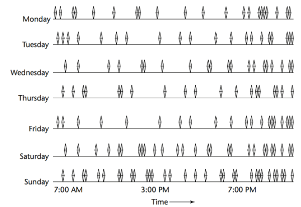
Figure 1: Varying arrival rate for customer orders
* Delivery service time, i.e., average time taken to deliver an order, and
* Number of FEs available at any given time.
Data analysis:
We have analyzed historic data related to arrival rates and service times for FD businesses and have made the following observations:
- Order Arrival Rate: The orders do not arrive at a uniform rate. In reality, customer arrival rate at a restaurant may look like this (Fig.1):
Figure 1: Varying arrival rate for customer orders
To model the incoming orders we assume a Markov process. According to the Markov process, the number of potential new customers is independent of the number of customers already waiting in the queue. A well-known Markov process that is often used to model the arrival rate of orders in a business such as the food delivery business is the Poisson process. According to this process, the number of new customers who arrive every hour is given by a Poisson distribution (see Appendix 1 for details). The main input parameter required to define a Poisson distribution is the average arrival rate per hour (λ), which is equal to 40 orders/hour for the example discussed above.
- Delivery Service Rate: Defined as the average number of customers served in an hour. This is dependent on the time is takes to serve a single order, which is a random variable, owing to unpredictable factors such as traffic conditions, wait times at the restaurant/customer, etc. As we write, we are collecting initial data from FD services and it appears that the service times follow a Gamma distribution with a mean of around 30 minutes (i.e., 2 order delivered per hour on average) and a standard deviation of 16.2 minutes (see Figure 2). These service times include the time it takes an FE to drive to the assigned restaurant, pick up the food, and deliver it to the customer.
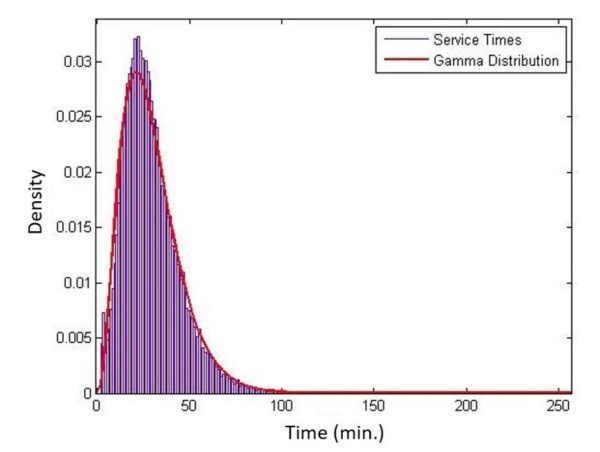
Fig 2: Service times follow a Gamma distribution with a mean of ~30 minutes and a standard deviation of 16.2 minutes
Based on the above observations, it is easy to understand why queues and waiting times build up for the food delivery business. If it was assumed that the arrival rates and service times are uniform, i.e., an order arrives every 1.5 minutes and it takes exactly 30 minutes to serve an order, then if we have more than 30/1.5 ~ 20 FEs, all orders will be processed immediately, without any queues being formed. However, due to the variability of arrival/service rates, a wait-free delivery service is not feasible.
Queuing System:
Now, to analyze the behavior of the queues being formed, we develop a queuing model based on the observed data, to help us estimate the average time a customer will need to wait before their order is delivered. Note that the wait time for a customer is defined as the sum of (i) the time the order is in queue, i.e., the time it takes for an order to be assigned to an FE (this happens when all FEs are busy with existing order deliveries), and (ii) the service time for the order (which follows a Gamma distribution).
Mathematically, the problem of assigning servers to customers falls under a class of problems known as “Queuing Problem” — literally, how the customers come and join a queue at irregular intervals and how do they get served. The queuing theory is not a hypothetical situation: lines in supermarkets or bus stations, or the waiting time for a person to respond when you call an airline, all follow queuing theory.
A queuing Model for our scenario will have the following structure (Fig. 3):
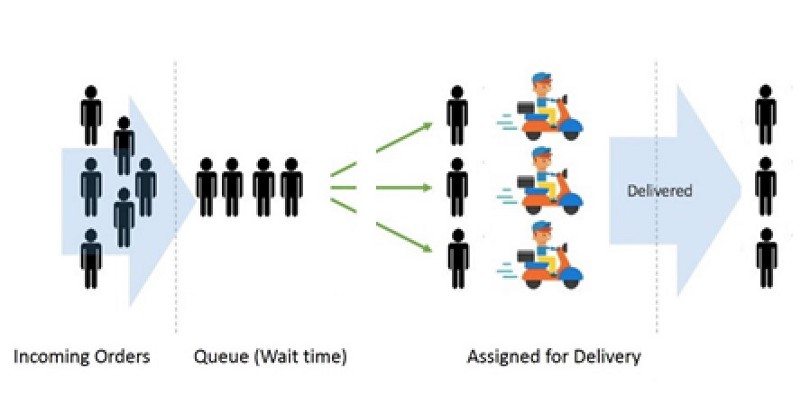
Figure 3: Typical food delivery process


- Incoming Orders: Orders arrive randomly and the number of orders per hour follow a Poisson distribution with a mean λ. The queuing system will be studied for different for different values of λ.
- Queue: The queue follows a First in First Out (FIFO) priority rule and is assumed to have an unlimited capacity, i.e., the food delivery business will not decline an order.
- Service: The serviceof the queuing system is dependent on the Number of FEs, the Service Rates, and the Order Aggregation Rate:
- The Number of FEs: We assume they all are equally good and take the same amount of time for an order completion.
- Service Rates: We know that service times are variable and follow a Gamma distribution with a mean of 30 minutes and standard deviation of 16.2 minutes. Thus, the mean service rate can be computed as µ = 2.
- Order Aggregation Rate: Defined as the fraction of all orders that are aggregated into shipments of two, e.g., when two orders are aggregated, the FE is able to deliver both of them in a single trip. If the order aggregation rate is high, it will improve the service rates as well. It can be easily derived that if a fraction x of all orders are aggregated into pairs, then the service rate µ will be multiplied by a factor of

- Current data suggests that less than 5% of orders are aggregated, implying that the updated service rate can be found as µ = 2.05.
Mathematical Description of the Proposed Queuing Model:
The above queuing model may be represented as an M/G/m model, in standard queuing nomenclature. “M” in the first field denotes that a Markov process is in place for the arrival rates; “G” in the second field denotes that a General distribution (Gamma in our case) is being used to model the service times; “m” in the third field denotes that multiple servers (FEs in our case) are being used in the queuing model.
This model is a somewhat exotic queuing model with very few analytical results available in the queuing literature. According to the research paper by Lee and Longton (1959), the mean waiting time for the M/G/m model can be approximated by using a factor to adjust the mean waiting time in an M/M/m queue. The latter model assumes that the service times follow an Exponential distribution and is among the most well studied queuing models in the literature. The formulae presented below represent the key metrics of the M/M/m queuing system and can be easily derived:
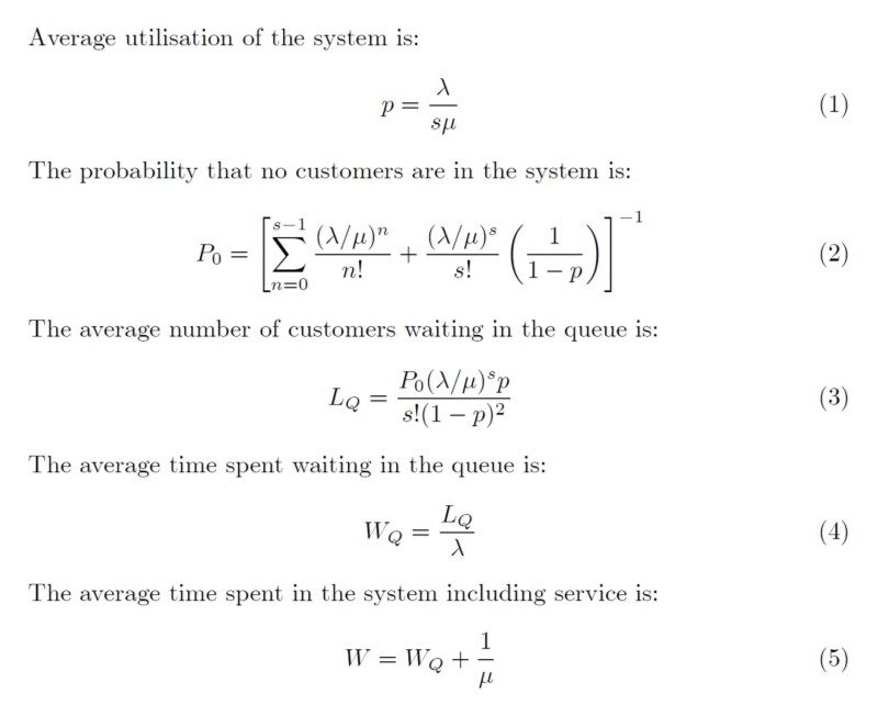
Finally, the mean time waiting time for the M/G/m model can be computed as:
![]()
![]()
where C is the coefficient of variation (ratio of standard deviation and mean, equal to 0.54 for our data) and W is the mean waiting time as found by formula (5).
Computational results: Wait times do not increase linearly
Using formula (6) for the average time spent in the system, we can compute the average time it takes for an order to be completed (service time + queue time) for varying arrival rates and the average utilization of the system (use formula (1)). It appears that the waiting time of the customers increase non-linearly with the arrival rates. Table 1 presents the results for a fixed number of FEs and several arrival rates.
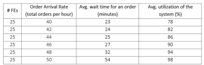
Table 1: Order Arrival Rate, Utilization and Customer Wait Time varies non-linearly
This is counter-intuitive: one would think that if a parameter changes by about 25% (in this case, arrival rate going up from 40 to 50), other associated parameters, such as waiting time would change in a similar manner, i.e., likely about 25% or so. Instead, the irregularity in the arrival rate makes the system highly unstable and increases wait time disproportionately, in this case, by 134%.
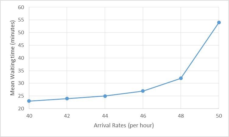
Figure 4: In this scenario, by increasing the number of customers from 40–50, i.e., just a change of 25%, mean waiting time goes from 23 minutes to 54 minutes
The Impact on P&L:
Table 2 shows FE salary bands for two types of scenario we encounter. In most cities the “Cost to Company (CTC)” for the FEs are Rs. 15,000 per month. In some parts of more expensive metros such as Bangalore and Delhi, the salaries are now inching up towards Rs. 18,000 per month. Note that a FD company has significant other expenses such as the fuel, bike rental, corporate overhead etc.
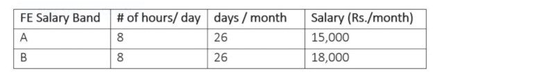
Table 2. Cost/FE for different salary bands
It can be easily understood that if we have more FEs on the ground, the average waiting time per order will be reduced. We currently promise a turn around time (TAT) of around 45 minutes. To meet this target on a consistent basis, the mean TAT should be around 30–35 minutes, as the standard deviation on the service times is around 16 minutes.
Let us see how many FEs are required to maintain a mean waiting time of about 30–35 minutes, for different arrival rates (see Table 3). For each arrival rate, we also show what happens when we have only one less FE than the recommended level. It turns out that the mean waiting time increases to about 55–60 minutes. If we take away another FE from the system, the delivery system becomes unfeasible, i.e., arrival rate becomes more than net service rate. These calculations are made using formula (6). Table 3 also provides the minimum amount that should be charged per order to attain profitability in each case.
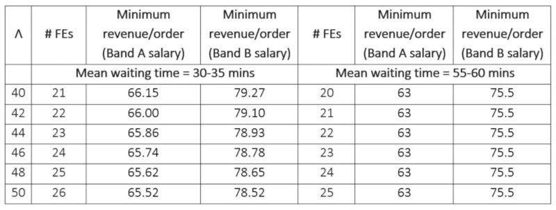
Table 3: Minimum number of FEs required for a given Arrival Rate and the corresponding revenue requirements per order (in Rs.); Λ represents the mean arrival rate per hour
Note that if the mean wait time is around 30 minutes (55 minutes), the minimum revenue requirement per order, hovers around Rs. 66 (Rs. 63)/order with Band A employees and around Rs. 79 (Rs. 76)/per order for Band B employees. In reality, the market does not allow us to charge more than Rs. 50 per order, thereby incurring losses on every order, even if we allow a mean wait time of 55–60 minutes, which may not be an acceptable turnaround time for food delivery orders.
Let us now scale up our calculations and calculate the “burn rate” assuming we aim for a mean wait time of around 30–35 minutes and the revenue per order is Rs. 50. Table 4 displays the “burn rate” under two scenarios:
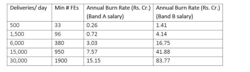
Table 4: Burn rate for a standalone FD company
Key Assumptions:
Notice that a number of key assumptions have been made in order to make the calculations presented in this article. All of these assumptions favor the FD business, so the results of the calculations should be seen as an optimistic estimate of the real situation. The main assumptions are:
- The mean arrival rate remains constant throughout the day — this is highly unlikely since in reality the order rate peaks only at meal times. Notice that the mean arrival rate of λ = 40 mentioned in the example discussed above, was for meal times only.
- The system has been optimized, so that as soon as the FE reaches the restaurant, the order is ready to be collected. In reality, this is extremely hard to achieve and it is often observed that the FE loses a lot of time (8 minutes on average) at the restaurant, while waiting for the food to be ready. For the purpose of our calculations, we have assumed this waiting time to be a nominal 2 minutes, since it is believed that with better scheduling of resources this wait time can be avoided.
- If two or more orders are aggregated, then an FE takes the same amount of time to deliver the aggregated order that it takes to deliver a single order.
Conclusion:
From our analysis, it is clear that the food delivery business is highly unstable, largely because the arrival/service rates of orders are not uniform. This results in large fluctuations in the delivery time, as well as utilization of the FEs, with high odds for unprofitability.
At the current scale, the order density is not very dense, which makes it difficult to aggregate orders and results in most orders being “Single pick, Single drop”. Our own internal data suggests that only about 4–5% orders are aggregated, which has little impact on the profitability of the FD model. However, if this figure increases to about 55%, calculations suggest that profitability may be achieved, provided all other assumptions still hold.
There are other potential ways to be profitable, for example, through cross-utilization of resources or with a different business model. A company that has multiple business lines such as food as well as package delivery, could cross-utilize the resources to build a profitable business model. For example, a package delivery company can use the FE’s for package delivery 9–12, some for Food Delivery 12–3, Package delivery 3–6 and some for food delivery at night.
A second alternative is a “food club” model with a limited menu and slotted delivery time. This takes out the uncertainties on the arrival rate out of the equation, resulting in high FE utilization.
A third alternative is an “in-house delivery person” model where an FE is also utilized for restaurant duties (such as food serving) to lower the overall cost of delivery and improve utilization. In reality, most Indian restaurants work on this model internally, so it might be worth understanding the economics of the same.
A fourth possible model is where the density of the users is high (such as Koramangala in Bangalore Metro Area), and food from a pre-selected menu is delivered within a very short period of time, something akin to what UberEATS is experimenting with.
The economics of the standalone food delivery lies in the science of incentives. If the current delivery rates charged by the existing FD cos are well below the cost borne internally, the entrepreneur will eventually shut down. On the other hand, if the price rises enough, the restaurant will likely switch to an in-house model.
Appendix 1:
Understand the Poisson distribution:
A Poisson process represents discrete events, like arrival of customers or phone calls at an exchange or a call center. As shown in the Fig. 5 below,N(t) = Number of arrivals in the time interval (0,t) is a random variable, which follows the Poisson distribution.
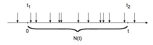
Figure 5: Number of arrivals in the time interval (0, t)
Mathematically, the probability of getting N(t) = x arrivals in a time window (0,t) can be given by,

where µ is the average number of arrivals in the time window (0,t).
The inter arrival times are independent and obey an exponential distribution, with mean inter arrival time (1/ µ) where µ is the arrival rate per unit time. For example, for an arrival rate of 40 customers per hour, µ =40. Figure 6 demonstrates this graphically.
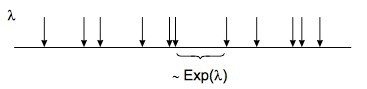
Figure 6: Inter-arrival times are independent and obey an exponential distribution
The epilogue:
The team that has worked on this post are Dr. Santanu Bhattacharya, Dr.Kabir Rustogi, Suvayu Ali (PhD candidate) and Snigdha Gupta, with active support from our CEO Sahil Barua and CTO Kapil Bharati. For full disclosure, Delhivery is India’s leading third party logistics provider. We work with many FD companies to help them gain efficiency.
The authors would like to thank numerous friends who have reviewed the paper and provided valuable feedback, including Nick Berry, Data Scientist at Facebook, Abhi Dhall of Multiples Equity, Ashok Tilotia of Kotak Security and Haresh Chawla of India Value Fund.
References:
- A. M. Lee and P. A. Longton, “Queueing Processes Associated with Airline Passenger Check-in,” Oper. Res. Quart. 10: 56–71 (1959)
[First published on Medium.]